测定总结
Brimrose ATOF-NIR自由空间光谱仪用于扫描含有不同量尼龙66,聚丙烯和丁苯,碳酸钙和三水合物的纤维样品,提供了5个样本,每个样本扫描5次。样品的大小和质地各不相同,从细粉到小块纤维,再到较大的地毯纤维。原始光谱数据经过处理后为吸收和第一导数。吸光度和第一个导数光谱被导入到化学测量软件中,创建了PLS 1回归模型,将光谱数据与尼龙6.6,聚丙烯和丁苯,碳酸钙和三水合物的百分比含量相关联。这个模型显示,光谱数据与参考值之间的相关性良好。
扫描了5个样本,但仅使用4个样本进行校准,因为对一个样本的参考值存在疑问。模型的载荷重量表明,模型的相关信息取自1700nm左右的C-H吸收区域和2050nm左右的C-O吸收区,这些是在测量这些参数时,人们期望能获取信息的波长区域。考虑到校准只使用了四个样品,并且所使用的光谱仪并没有针对此应用进行优化,因此测试结果应该说特别好。本研究的结果基于,当可以使用更多样本,使用扫描收集光谱数据时与样品接触的手持光谱仪。
总的来说,本研究证明了使用Brimrose AOTF-NIR近红外光谱仪收集的光谱数据测量尼龙66,聚丙烯和丁苯,碳酸钙和三水合物的可行性。
总结介绍
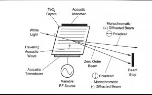
AOTF的原理是基于光在各向同性介质中的声衍射,该装置由一个压电传感器与一个双折射仪连接在一起构成,当传感器被应用的射频信号激活时,会在晶体中产生声波。传播声波产生了折射率的周期性调制,这提供了一个移动光栅,在适当的条件下,会衍射部分入射光束。对于固定声频,窄频段的光频满足匹配条件,并累积衍射。随着RF频率的变化,光带的中心也会相应地改变,从而保持相位匹配条件。
The near infrared region of the spectrum extends from 800nm to 2500nm. The absorption bands that are most prominent in this region are due to overtones and combinations of the fundamental vibrations active in the mid-infrared region. The energy transitions are
between the ground state and the second or third excited vibrational states. Because higher energy transitions are successively less likely to occur, each overtone is successively weaker in intensity. Because the energy required to reach the second or third excited state is approximately twice or three times that needed for a first order transition and the wavelength of absorption is inversely proportional to the energy, the absorption bands occur at about one-half and one-third the wavelength of the fundamental. In addition to the simple overtones, combination bands also occur. These usually involve a stretch plus one or more bending of rocking modes. Many different combinations are possible and therefore the NIR region is complex, with many band assignments unresolved.
Near Infrared Spectroscopy is currently being used as a quantitative tool that relies on chemometrics to develop calibrations relating a reference analysis of the constituent to that of the NIR optical spectrum. The mathematical treatment of NIR data includes Multi Linear Regression (MLR), Principle Component Analysis (PCR), Partial Least Squares (PLS) and discriminant analysis. All of these algorithms can be used singularly or in combination to yield the resultant goal of quantitative prediction and qualitative description of the constituents of interest.
III. Methodology
A Brimrose AOTF-NIR Free Space spectrometer was used to scan five samples with containing varying amounts of Nylon 6,6, Polypropylene & Styrene Butadiene, and Calcium Carbonate & Aluminum Tri-Hydrate. Five different portions of each sample were scanned. Wavelength range was from 1100nm to 2300nm with 2nm resolution. One hundred scans were collected per reading and averaged into one spectrum. The raw spectral data were post-processed into absorbance and first derivative. The absorbance and first derivative spectra were imported into the chemometrics software program The Unscrambler. The first derivative spectra were used to create PLS 1 regression models for N66, PP & SB, and CC & AlTH. It was noted that the reference values for Sample 2 may have been erroneous. When the samples were shipped, nominal values for the parameters were provided. Sample 2 had an estimated value of 38%-42% for N66, 38%-42% for PP, and 20%-24% for CC & AlTH. When the actual sample values were provided for Sample 2, N66 had a value of 62.6%, PP & SB had a value of 25.4%, and CC & AlTH had a value of 12.0%. The reasons for the discrepancies were unclear but the models for all three parameters showed better results when the data points from Sample 2 were removed. One possible reason is that Sample 2 was made up of much larger pieces of fiber than the other samples. The variance of reference values within the given sample may have been much higher than the variance in the other samples. Thus, all models shown here do not have data points from Sample 2
Results
- Spectra
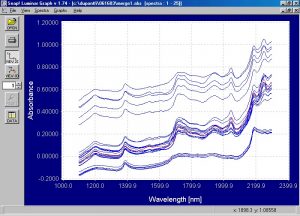
There is a clear baseline shift effect in the spectra due to differences in the distance of the samples from the optical head of the Free Space spectrometer. Chemometric modeling handles baseline shifts well and a hand-held spectrometer that is in contact with the samples when scanning will greatly reduce this effect. The following graph shows the first derivative spectra of the samples.
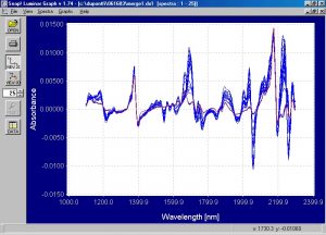
The first derivative spectra eliminate the baseline shift effect and make the spectral differences between the samples much clearer. The differences between Sample 5 and the rest of the samples are especially clear. The Sample 5 spectra are shown in red on the graph. This sample contains a much higher % CC & AlTH and lower %N66 and %PP & SB than the other samples. The differences are most clear around 1700nm, 2050nm, and 2250nm. The regression models will show that these wavelength areas are important areas in the models. The first derivative spectra were used to create regression models for N66, PP & SB, and CC & AlTH. Modeling results are shown in the graphs below.
- Modeling and Regressions
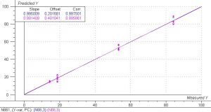
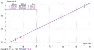
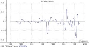
The regression model for N66 showed good correlation between the spectral data and reference values, especially considering the small amount of samples used in the study. The calibration and validation correlation coefficients are high at 0.997 and 0.995. Three principle components were used. The Standard Error of Prediction (SEP) is equal to 2.5. This error will be reduced when more samples are used over the entire range of values. There is also some spread in some of the data points and this effect will be reduced when a hand-held spectrometer that is in contact with the samples during scanning is used. The high correlation coefficients indicate that the model does obtain correlation from the spectral data and that the error will be less when more samples are used for the calibration. The graph below shows the loading weights plot for the N66 model.
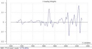
Peaks (positive or negative) in a loading weights plot for a PLS 1 regression model show the wavelengths that contain relevant information for the model. The plot for the N66 shows peaks in the C-H absorbing areas around 1700nm and 2250nm and the C=O area around 2050nm. These are also the wavelength ranges where visible spectral differences are seen in the first derivative spectra and ranges where one would expect to see spectral changes due to changes in N66.
The regression model for PP & SB showed good correlation between the spectral data and reference values, especially considering the small amount of samples used in the study. The calibration and validation correlation coefficients are high at 0.998 and 0.997. Two principle components were used. The Standard Error of Prediction (SEP) is equal to 0.8. This error will be reduced when more samples are used over the entire range of values. There is also some spread in some of the data points and this effect will be reduced when a hand-held spectrometer that is in contact with the samples during scanning is used. The high correlation coefficients indicate that the model does obtain correlation from the spectral data and that the error will be less when more samples are used for the calibration. The graph below shows the loading weights plot for the PP & SB model.
Peaks (positive or negative) in a loading weights plot for a PLS 1 regression model show the wavelengths that contain relevant information for the model. The plot for the PP & SB model shows peaks in the C-H absorbing areas around 1700nm and 2250nm. These are also wavelength ranges where visible spectral differences are seen in the first derivative spectra and ranges where one would expect to see spectral changes due to changes in PP. There is no peak at 2050nm and this is further proof that the model is fitting relevant information because PP contains no C=O bonds.
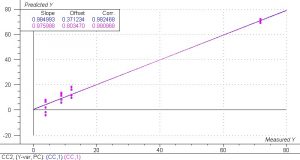
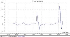
The regression model for CC & AlTH showed good correlation between the spectral data and reference values, especially considering the small amount of samples used in the study. The calibration and validation correlation coefficients are high at 0.992 and 0.990. One principle component was used. The Standard Error of Prediction (SEP) is equal to 3.4. This error will be reduced when more samples are used over the entire range of values. There was an especially large difference between the high sample value (71.5%) and the low sample values. There is also some spread in some of the data points and this effect will be reduced when a hand-held spectrometer that is in contact with the samples during scanning is used. The high correlation coefficients indicate that the model does obtain correlation from the spectral data and that the error will be less when more samples are used for the calibration. The graph below shows the loading weights plot for the CC & AlTH model.
Peaks (positive or negative) in a loading weights plot for a PLS 1 regression model show the wavelengths that contain relevant information for the model. The plot for the CC and AlTH model shows peaks in the C-H absorbing areas around 1700nm and 2250nm and the C=O bond absorbing area around 2050nm. Calcium carbonate does contain carbon-oxygen bonds but no C-H stretches. However, the fact that the other two components in the samples do contain C-H stretches means that an indirect correlation can be obtained in these wavelength ranges for CC & AlTH. The wavelength ranges where visible spectral differences are seen in the first derivative spectra and ranges where one would expect to see spectral changes due to changes in CC & AlTH.
Discussion and Conclusions
The results of this study proved the feasibility of measuring Nylon 6,6, Polypropylene & Styrene Butadiene, and Calcium Carbonate & Aluminum Tri-Hydrate from spectral data collected using a Brimrose AOTF-NIR Free Space spectrometer and calibration models. The correlation coefficients for the models were high and there are many ways that the results obtained in this study can be improved upon. When the data from Sample 5 was taken out of the models, there were only four samples used in the study and these samples had many differences in fiber size and texture. The results will improve when more samples over the full range of reference values for all three parameters are added to the calibration models. The results obtained here should also improve when a hand-held spectrometer that comes into contact with the samples is used. There were some variations in the distance of the samples to the optical head of the Free Space spectrometer and this may have contributed to some of the error. Past experience has shown that using one hundred or more samples for a calibration model will increase model robustness and reduce prediction error. Past experience has also shown that the results of a study conducted in the laboratory can be duplicated in a real-life, on-line situation.
The Brimrose AOTF-NIR spectrometer is the ideal tool for real-time, on-line measurements. Fast, accurate readings can be obtained using no moving parts and without the need to recalibrate the system. In this case, calibration models can be created for each of the parameters measured in this study. Once the models are created, a hand-held spectrometer can be used to scan samples and obtain readings for N66, PP & SB, and CC & AlTH. Overall, this study proved the feasibility of measuring N66, PP & SB, and CC & AlTH from spectral data collected using a Brimrose AOTF-NIR spectrometer. It is recommended that a discussion be held to determine the best method for implementing a Brimrose AOTF-NIR Luminar 4030 hand-held spectrometer for real-time measurement of these parameters.