Brimrose AOTF-NIR光谱仪测定树脂对硬化剂的百分比
I. 简介
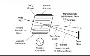
声光可调滤波器(AOTF)的原理基于光在各向异性介质中的声折射。装置由粘在双折射晶体上的压电导层构成。当导层被应用的射频(RF)信号激发时,在晶体内产生声波。传导中的声波产生折射率的周期性调制。这提供了一个移动的相栅,在特定条件下折射入射光束的部分。对于一个固定的声频,光频的一个窄带满足相匹配条件,被累加折射。RF频率改变,光的带通中心相应改变以维持相匹配条件。
光谱的近红外范围从800nm到2500 nm延伸。在这个区域最突出的吸收谱带归因于中红外区域的基频振动的泛频和合频。是基态到第二激发态或第三激发态的能级跃迁。因为较高能级跃迁连续产生的概率较小,每个泛频的强度连续减弱。由于跃迁的第二或第三激发态所需的能量近似于第一级跃迁所需能量的二倍或三倍,吸收谱带产生在基频波长的一半和三分之一处。除简单的泛频以外,也产生合频。这些通常包括延伸加上一个或多个振动方式的伸缩。大量不同合频是可能的,因而近红外区域复杂,有许多谱带彼此部分叠加。
现在,NIRS被用作定量工具,它依赖化学计量学来发展校正组成的参照分析和近红外光谱的分析的关联。近红外数据的数学处理包括多元线性回归法(MLR)、主成分分析法(PCA)、主成分回归法(PCR)、偏最小二乘法(PLS)和识别分析。所有这些算法可以单独或联合使用来得到有价值组成的定性描述和定量预测。
II. 测量方法
- Sample Preparation
Brimrose was supplied with approximately 300ml of a polyester resin solution labeled COAT1 and approximately 100 ml of a polyisocyanate solution labeled CO-REACTANT 1. Because both solutions were too viscous to be drawn through a measuring pipette, an alternate method for measuring out proportions was used. Using a measuring pipette, 10mL of ethyl acetate was measured and dispensed into a small 15mL vial and the level obtained was marked. This procedure was repeated for each vial. Each vial was then filled to this mark with the polyester resin. A similar procedure was used to measure the more viscous co-reactant. The ends of the plastic pipette tips were enlarged by clipping off approximately 5mm of the tip, so that the co-reactant could be drawn into them. An amount of ethyl acetate was drawn into the pipette tip and the level marked. This was done for each sample prepared as a secondary assurance that the proper amount of co-reactant was being drawn into the pipette tip (see Tables 1 and 2 for prepared samples). Twenty five percent of the co-reactant is ethyl acetate. In order to obtain a true percent volume of the co-reactant in each sample the 25% ethyl acetate was first factored out. The product was then divided by the total volume and multiplied by a constant of 10. A chemical reaction begins to take place upon mixing of the two solutions and spectra were immediately collected.
| Sample | COAT1 | Co-reactant | % Co-reactant |
| S-01 | 10ml | 0.600ml | 0.42 |
| S-02 | 10ml | 0.550ml | 0.39 |
| S-03 | 10ml | 0.530ml | 0.38 |
| S-04 | 10ml | 0.500ml | 0.36 |
| S-05 | 10ml | 0.480ml | 0.34 |
| S-06 | 10ml | 0.450ml | 0.32 |
| S-07 | 10ml | 0.430ml | 0.31 |
| S-08 | 10ml | 0.400ml | 0.29 |
| S-09 | 10ml | 0.380ml | 0.27 |
| S-10 | 10ml | 0.350ml | 0.25 |
| S-11 | 10ml | 0.330ml | 0.24 |
| S-12 | 10ml | 0.300ml | 0.22 |
| S-13 | 10ml | 0.280ml | 0.20 |
| S-13A | 10ml | 0.280ml | 0.20 |
| S-14 | 10ml | 0.250ml | 0.18 |
| S-14A | 10ml | 0.250ml | 0.18 |
| S-15 | 10ml | 0.550ml | 0.39 |
| S-16 | 10ml | 0.600ml | 0.42 |
| S-16A | 10ml | 0.600ml | 0.42 |
Table 1. Calibration Set
| Sample | COAT1 | Co-reactant | % Co-reactant |
| VAL-17 | 10ml | 0.570ml | 0.40 |
| VAL-18 | 10ml | 0.520ml | 0.37 |
| VAL-18 | 10ml | 0.520ml | 0.37 |
| VAL-19 | 10ml | 0.460ml | 0.33 |
| VAL-19 | 10ml | 0.460ml | 0.33 |
| VAL-20 | 10ml | 0.4150ml | 0.30 |
| VAL-20 | 10ml | 0.415ml | 0.30 |
Table 2. Validation Set
- Data Collection
A Brimrose AOTF-NIR Luminar spectrometer was used for data collection. Spectra were collected in transmission mode using fiber optic cable with 600mm diameter low OH Silica core. The spectral range was 900nm to 1700nm with a 2nm resolution. The effective path-length was 10mm. Spectra were also collected on the raw solutions.
III. Results
- Spectra
The absorbance spectra of the raw solutions are shown below in Figure 2. These spectra show clearly the areas of each solution that absorb differently. Figure 2 shows that the co-reactant absorbs quite strongly between 1450nm and 1600nm, while the polyester resin has no absorbing properties in the same region. This will prove to be an important region when modeling the data and will be discussed later in this report. There is a slight difference between the absorbing characteristics of the resin and the co-reactant at 1384nm. It is clear that the resin has a stronger absorbing peak at 1177nm. These two areas of the spectral range will also show to be important when modeling the data.
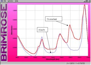
Figure 2. Absorbance spectra of raw solutions
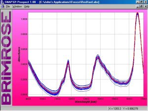
Figure 3. Absorbance spectra of mixed COAT1 and co-reactant solutions
Initially 16 samples were prepared. An aliquot of samples S-13, S-14, and S-16 were scanned and added into the calibration for a combined total of 19. Spectra of the 19 samples are shown in Figure 3. Later 4 additional samples with proportions not represented in the calibration set were prepared and scanned. An aliquot of VAL-18, VAL-19 and VAL-20, for a total of 7 samples in the validation set, were also scanned and included in the total matrices (see Table 2).
- Modeling and Regressions
There were a total of 26 spectra, which were imported as absorbance data into the chemometrics software package The Unscramblerä. As stated earlier in this report, the complete wavelength range was from 900nm to 1700nm. For modeling purposes, different wavelength regions were examined in an attempt to obtain the best results. After analyzing the spectra and performing regressions on several different regions, the region between 1172nm and 1620nm was found to give the best results. Sample S-03 was considered a highly influential outlier due to both high residual Y variance and leverage and was not included in the regression. The regression is shown below in Figure 4. With sample S-03 removed, the regression shows very good correlation between X (spectra) and Y (response or measured) data. This holds true for both the calibration and validation. Correlation values were 0.97 and 0.95 respectively. The SEP (standard error of prediction) and SEC (standard error of calibration) was 0.028 and 0.022 respectively.
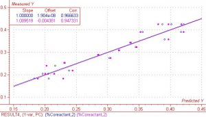
Figure 4. Regression on % co-reactant with one outlier removed.
As previously mentioned, the region between 1450nm and 1600nm is an area in which the COAT1 solution does not absorb and the co-reactant absorbs quite strongly. This same wavelength region results in very high regression coefficients and X loading, which indicates there is information in the spectral data that correlates well to the measured Y response values. Regression coefficients and X loading are shown below in Figures 5 and 6 respectively. Although not quite as pronounced, the regression coefficients and X loading are slightly higher in the other two spectral regions of interest, i.e. 1384nm and 1177nm.
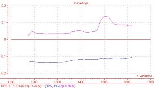
Figure 5. X – Loading for PC’s 1 and 2
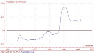
Figure 6. Regression coefficients for second Principle Component
- Prediction
A model built from 18 calibration samples, which excluding sample S-03 was applied to the 7 samples mixed and retained for validating the model. These samples are identified as such in Table 2. The SEP for the Validation set was 0.026 and agrees quite closely with 0.027 given for the model. Prediction results can be seen in Table 3 below.
| % Co-Reactant by Volume | |||
| Sample | Predicted | Measured | Difference |
| VAL-17 | 0.414 | 0.40 | 0.010 |
| VAL-18 | 0.361 | 0.37 | -0.010 |
| VAL-18 | 0.358 | 0.37 | -0.013 |
| VAL-19 | 0.342 | 0.33 | 0.012 |
| VAL-19 | 0.392 | 0.33 | 0.062 |
| VAL-20 | 0.336 | 0.30 | 0.037 |
| VAL-20 | 0.308 | 0.30 | 0.009 |
| SEP= | 0.026 | ||
Table 3. Prediction result on % co-reactant
- Conclusion
The results of this feasibility study indicate that the determination of % co-reactant in a mixture with COAT1 is very feasible using the Brimrose AOTF-NIR Luminar spectrometer. However, better results could be obtained by using a larger calibration set of approximately 40 samples in a laboratory with tools that allow for more accurate measurements. There were many unavoidable errors because of the limited resources available for doing this experiment. This is especially true for the more viscous co-reactant. It was necessary to first measure a volume of solvent and then pour this amount in a vial. The volume amount was then marked on the vial. The COAT1 was then poured into the vial and brought to the mark. This two step process increased the amount of error associated with measuring precise amounts. The same procedure was used for the more viscous co-reactant but the error factor was even greater. A certain amount was lost because the pipette tip could not be completely rinsed of the co-reactant. Another error factor was that a given amount of the co-reactant clung to the outside of the pipette and was unavoidably dissolved into the mixture. A third way of introducing error was in the size of the samples. Because none of the samples was greater than 10.6mL, any error in measurement will by compounded by the use of such small samples. Making corrections to the error factors in this experiment should result in obtaining a more precise calibration set which will create a more robust model that is able to predict with greater accuracy.