Brimrose AOTF-NIR光谱法快速鉴别回收利用的聚合物废弃物
I. 简介
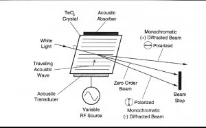
声光可调滤波器(AOTF)的原理基于光在各向异性介质中的声折射。装置由粘在双折射晶体上的压电导层构成。当导层被应用的射频(RF)信号激发时,在晶体内产生声波。传导中的声波产生折射率的周期性调制。这提供了一个移动的相栅,在特定条件下折射入射光束的部分。对于一个固定的声频,光频的一个窄带满足相匹配条件,被累加折射。RF频率改变,光的带通中心相应改变以维持相匹配条件。
光谱的近红外范围从800nm到2500 nm延伸。在这个区域最突出的吸收谱带归因于中红外区域的基频振动的泛频和合频。是基态到第二激发态或第三激发态的能级跃迁。因为较高能级跃迁连续产生的概率较小,每个泛频的强度连续减弱。由于跃迁的第二或第三激发态所需的能量近似于第一级跃迁所需能量的二倍或三倍,吸收谱带产生在基频波长的一半和三分之一处。触简单的泛频以外,也产生合频。这些通常包括延伸加上一个或多个振动方式的伸缩。大量不同合频是可能的,因而近红外区域复杂,有许多谱带彼此部分叠加。
现在,NIRS被用作定量工具,它依赖化学计量学来发展校正组成的参照分析和近红外光谱的分析的关联。近红外数据的数学处理包括多元线性回归法(MLR)、主成分分析法(PCA)、主成分回归法(PCR)、偏最小二乘法(PLS)和识别分析。所有这些算法可以单独或联合使用来得到有价值组成的定性描述和定量预测。
II.实验方法
- 仪器设备
水平安装Brimrose 自由空间光谱仪的光学模块,只需要将光学模块贴近玻璃窗口就可以查看样品。窗口被一个架子支撑在支架上,与模块在合适的距离。这种架构模拟了真实的生产场景。
- 数据收集
The spectra from soft back samples of carpets were collected once from the shag side and once from the back side to simulate a real life situation where pieces may face the spectrometer either way. The spectra from yarn samples was collected once, without any attempt to create a reproducible packing density, again assuming that in real life yarns will be presented with variability of the conditions. The hard waste in form of chips, flakes or pellets was loaded into petri dishes and spectra was collected in a static mode for a fraction of a second (10 scans). This condition creates spectra collection that is more difficult to use because it represents a smaller number of pieces. In real life the situation will be better because the sample will be moving and the spectrometer will collect spectra on a larger sample.
III. Results
- Spectra
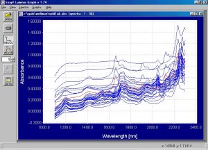
Figure 2. Absorbance spectra from soft back and yarn samples of N66, N6, polypropylene and PET.
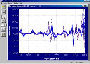
Figure 3. First derivative spectra from samples shown in absorbance spectra above.
The differences become much more apparent in the first derivative spectra than in the absorbance spectra.

Figure 4. Absorbance spectra from solid waste samples. The spectrum from the sample PPSC002 (PET clear film) is the one on the bottom, showing the “sinusoidal” shape that is typical of interference fringes behavior. The second spectrum from the top that shows very flat response is the one from sample NXBC002, the high carbon containing nylon.
The spectra basically are similar to that of the soft waste and the physical shape of the samples and the differences in packing density do not affect the ability to collect acceptable spectra. The only difficulty experienced with the hard waste was with the samples that contained a high degree of carbon powder because these samples absorb the NIR light very strongly. As a result, the conditions that are suitable for collecting from regular waste are not adequate for those with carbon filler. The other type of sample that created problems was the fine sheet film. This sample responded as expected with spectra that show the phenomenon known as “interference fringes”. It is possible that if such waste becomes very dense due to packing pressure in the container, this issue will be resolved. If not, other approaches will be examined to resolve the issue.
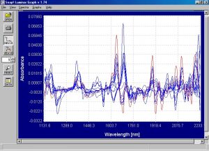
Figure 5. First derivative spectra from the absorbance spectra from Figure 4.
As was the case with the soft waste, the spectral differences become more apparent when looking at the first derivative spectra. Although it is not completely apparent by sight, the first derivative spectra from the clear film is completely meaningless.
- Regressions, Modeling, and Predictions
In order to evaluate the ability to distinguish between the nylons, the polypropylene (PP) and the PET samples, an arbitrary number was assigned to each group. The PET’s were given a value of one, the PP were given a value of 2, and the nylons a value of 3. A PLS 1 regression was run using the chemometric software package Unscrambler. The regression is shown in Figure 6 below.

Figure 6. PLS 1 regression model of the arbitrary values for the different polymers.
The standard error of prediction (SEP) is only 0.16, indicating a very good regression. Considering the fact that there were only a small number of PP samples, the “drift” of the PP samples to the left of the line can be understood. A larger number of PP samples are needed for a better regression. Despite this, the distinction between the PP, PET and nylons is complete.

Figure 7. Regression coefficients for the regression shown in Figure 6 above.
The regression coefficients show the wavelength regions from where the model gets its relevant information. It is pretty clear that the regression coefficients correspond to the wavelength regions in the first derivative spectra where the largest changes occur. This is one indication that the model is a good one and that the spectral information comes from relevant wavelength regions where changes occur. This model was used to predict values for the unknowns and the results are shown in the table below.
| Sample name | Prediction | Sample name | Prediction |
| SB010 | Nylon | Y056 | Nylon |
| SB011 | Nylon | Y073 | Nylon |
| SB050 | Nylon | Y028 | Nylon |
| SB047 | Nylon | NET#1 | Nylon |
| SB005 | Nylon |
NET#2 |
Nylon |
| SB006 | Nylon | NET#3 | Nylon |
| SB024 | Nylon | NCRE004 | Nylon |
| SB026 | Nylon | NPO057 | PET |
| Y023 | Nylon | NPO050 | PET |
| Y045 | Nylon | NPO062 | PET |
| Y061 | Polypropylene | NN058 | Nylon |
| Y037 | Nylon | NN067 | Nylon |
| Y007 | Nylon | NN066 | Nylon |
| Y027 | Nylon |
Table 1. Prediction of unknown samples on the basis of regression between the nylons as one group.
The predictions of all samples were correct. However, because the chemical differences between the two nylon types (6 and the 6,6) are much smaller than the differences between the three types, it is not realistic that a general model covering all three polymers will predict between the two nylons. In order to verify the validity of the method for these two types of nylon a sub-set of samples containing only nylons was created. In this set, nylon 6 was given a value of 1 and nylon 6,6 was given a value of 2. A regression model was created and the result is shown in Figure 8 below. The SEP is only 0.145 and it is definitely indicative that distinguishing between the two nylon types is feasible with high degree of reliability. To test the reliability of the method, several sets of “unknowns” were created, by removing some samples from the regression. These “unknowns” were then predicted along with the real unknowns.
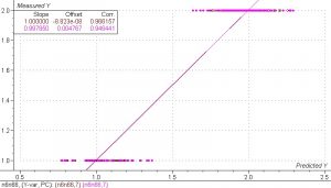
Figure 8. PLS 1 regression model of nylon 6 and nylon 6,6 samples. The SEP is only 0.145. The results suggest that distinguishing between the two nylon types is very feasible.
The results for this model were excellent. The SEP is very low and indicates that separating the two nylon types is definitely feasible. Several sets of artificial unknowns are shown in the table below. With the possible exception of sample Y004, all the predictions are correct. It is very possible that this sample was mislabeled as Nylon 6,6 when it was actually Nylon 6.
This table shows validation sets 1 through 5. The real unknowns are listed first and they were predicted very reproducibly in all 5 sets.
| Sample | Predict | Status | Sample | Predict | Status |
| Ncre004 | 6,6 | V | Y015 | 6,6 | + |
| Net#1 | 6,6 | V | Y022 | 6,6 | + |
| Net#2 | 6,6 | V | Y044 | 6 | + |
| Net#3 | 6,6 | V | Y046 | 6,6 | + |
| SB005 | 6 | V | Y059 | 6,6 | + |
| SB006 | 6,6 | V | Y072 | 6,6 | + |
| SB010 | 6,6 | V | Y086 | 6 | + |
| SB011 | 6,6 | V | Nmil017 | 6,6 | + |
| SB024 | 6,6 | V | SB002 | 6,6 | + |
| SB026 | 6,6 | V | SB007 | 6,6 | + |
| SB047 | 6,6 | V | SB040 | 6 | + |
| SB050 | 6,6 | V | SB046 | 6,6 | + |
| SB055 | 6 | V | SB053 | 6 | + |
| Y007 | 6 | V | SB064 | 6 | + |
| Y023 | 6,6 | V | SB065 | 6,6 | + |
| Y027 | 6,6 | V | Y002 | 6 | + |
| Y028 | 6,6 | V | Y006 | 6 | + |
| Y037 | 6,6 | V | Y024 | 6,6 | + |
| Y045 | 6,6 | V | Y031 | 6,6 | + |
| Y056 | 6,6 | V | Y040 | 6,6 | + |
| Y073 | 6 | V | Y068 | 6,6 | + |
| Artificial unknowns | Y077 | 6,6 | + | ||
| Nab002 | 6,6 | + | YSBO699 | 6 | + |
| SB001 | 6,6 | + | SB028 | 6,6 | + |
| SB008 | 6,6 | + | SB035 | 6,6 | + |
| SB015 | 6 | + | SB060 | 6,6 | + |
| SB019 | 6 | + | SB062 | 6,6 | + |
| SB023 | 6 | + | Y026 | 6,6 | + |
| SB030 | 6,6 | + | Y049 | 6,6 | + |
| SB034 | 6,6 | + | Y063 | 6,6 | + |
| SB041 | 6,6 | + | Y072 | 6,6 | + |
| Y005 | 6,6 | + | SB013 | 6 | + |
| SB027 | 6,6 | + | Y076 | 6,6 | + |
| SB041 | 6,6 | + | NBS2065 | 6,6 | + |
| SB057 | 6 | + | NWTX012 | 6,6 | + |
| Y001 | 6 | + | SB008 | 6,6 | + |
| Y022 | 6,6 | + | SB016 | 6 | + |
| Y030 | 6 | + | SB019 | 6 | + |
| Y062 | 6,6 | + | SB025 | 6 | + |
| Y067 | 6,6 | + | SB030 | 6,6 | + |
| Y069 | 6,6 | + | SB043 | 6,6 | + |
| Y029 | 6,6 | + | Y054 | 6,6 | + |
| Y069 | 6,6 | + | YBSO716 | 6 | + |
| Y071 | 6,6 | + | Y010 | 6 | + |
| Y004 | 6 | (-) | |||
Table 2. Prediction results of real unknowns and artificial unknowns based on 5 sets of regressions where the unknowns were kept out of the regression and predictions were made using the model. A V sign stands for correct prediction of a real unknown. A + sign stands for correct prediction of a known sample that was treated as an unknown by keeping it out of the calibration set.
One can see that sample Y004 was labeled 6,6 and it was predicted twice as 6, using two different sets of artificial unknowns. It is possible that it was mislabeled and should be checked again.
B. Hard waste
The hard waste spectra, without the spectra for the very dark nylon pellets, and the thin clear film that produced the poor spectra discussed above was subjected to chemometric treatment. The result is similar, and despite the large differences in the physical shape of the samples, from chunks to flakes, the regression only required 2 PC’s. It is obvious to Brimrose that a larger sample set will give even better results.
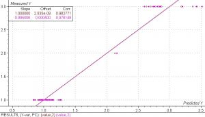
Figure 9. PLS 1 regression model of the nylon (6 and 6,6), polypropylene and PET with arbitrary values of 3, 2 and 1 respectively. The SEP is only 0.18, and only 2 PC’s were used.
Due to the small number of samples of nylon 6 among the nylon samples it was not possible to perform a separate regression to show the feasibility of distinguishing between the two nylons. However, it is expected that the results will be similar to the soft-back. From an operational point of view, it is preferable to have the large chunks hard waste shredded prior to presentation to the spectrometer simply because it will provide better spectra.
IV. Conclusions and Recommendations
It can be concluded from the results of this experiment that it is definitely feasible to separate and identify these types of polymers using the Brimrose AOTF-NIR spectrometer. The nylons can be separated from the PET and PP and the nylons can be separated from each other using separate regression models. The speed of the Brimrose instrument will enable the identification to be done quickly, most likely at a rate of 3-5 times per second on waste moving in a chute. A Brimrose Free Space spectrometer can be installed on a chute where the waste is being loaded or unloaded as the waste is moving. The results can be displayed on a monitor in the operator’s control room. A Macro program can be written that when used with the Brimrose SNAP! Software will enable the design of alarms for when the presence of an undesired polymer mixed with a desired polymer exceeds a certain level.